Activate

$n$-Cube

This section provides some examples on Chapter 2 of Stanley’s book [Stanley2013], which deals with $n$-cubes, the Radon transform, and combinatorial formulas for walks on the $n$-cube.

The vertices of the $n$-cube can be described by vectors in $\mathbb{Z}_2^n$. First we define the addition of two vectors $u,v \in \mathbb{Z}_2^n$ via the following distance:

sage: def dist(u,v):
....:     h = [(u[i]+v[i])%2 for i in range(len(u))]
....:     return sum(h)

The distance function measures in how many slots two vectors in $\mathbb{Z}_2^n$ differ:

sage: u=(1,0,1,1,1,0)
sage: v=(0,0,1,1,0,0)
sage: dist(u,v)
2

Now we are going to define the $n$-cube as the graph with vertices in $\mathbb{Z}_2^n$ and edges between vertex $u$ and vertex $v$ if they differ in one slot, that is, the distance function is 1:

sage: def cube(n):
....:     G = Graph(2**n)
....:     vertices = Tuples([0,1],n)
....:     for i in range(2**n):
....:         for j in range(2**n):
....:             if dist(vertices[i],vertices[j]) == 1:
....:                 G.add_edge(i,j)
....:     return G

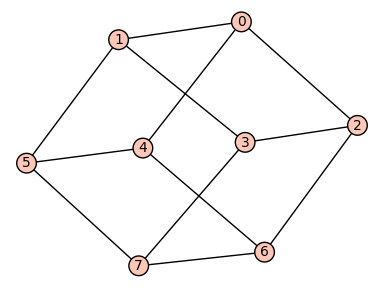
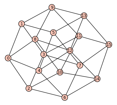
We can plot the $3$ and $4$-cube:

sage: cube(3).plot()
Graphics object consisting of 21 graphics primitives

sage: cube(4).plot()
Graphics object consisting of 49 graphics primitives

Next we can experiment and check Corollary 2.4 in Stanley’s book, which states the $n$-cube has $n$ choose $i$ eigenvalues equal to $n-2i$:

sage: G = cube(2)
sage: G.adjacency_matrix().eigenvalues()
[2, -2, 0, 0]

sage: G = cube(3)
sage: G.adjacency_matrix().eigenvalues()
[3, -3, 1, 1, 1, -1, -1, -1]

sage: G = cube(4)
sage: G.adjacency_matrix().eigenvalues()
[4, -4, 2, 2, 2, 2, -2, -2, -2, -2, 0, 0, 0, 0, 0, 0]

It is now easy to slightly vary this problem and change the edge set by connecting vertices $u$ and $v$ if their distance is 2 (see Problem 4 in Chapter 2):

sage: def cube_2(n):
....:     G = Graph(2**n)
....:     vertices = Tuples([0,1],n)
....:     for i in range(2**n):
....:         for j in range(2**n):
....:             if dist(vertices[i],vertices[j]) == 2:
....:                 G.add_edge(i,j)
....:     return G

sage: G = cube_2(2)
sage: G.adjacency_matrix().eigenvalues()
[1, 1, -1, -1]

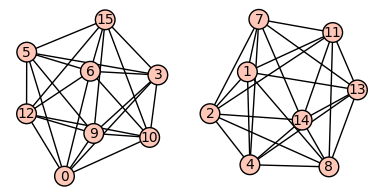
sage: G = cube_2(4)
sage: G.adjacency_matrix().eigenvalues()
[6, 6, -2, -2, -2, -2, -2, -2, 0, 0, 0, 0, 0, 0, 0, 0]

Note that the graph is in fact disconnected. Do you understand why?

sage: cube_2(4).plot()
Graphics object consisting of 65 graphics primitives